Got a Scatter Plot? Learn How to Add Marginal Histograms
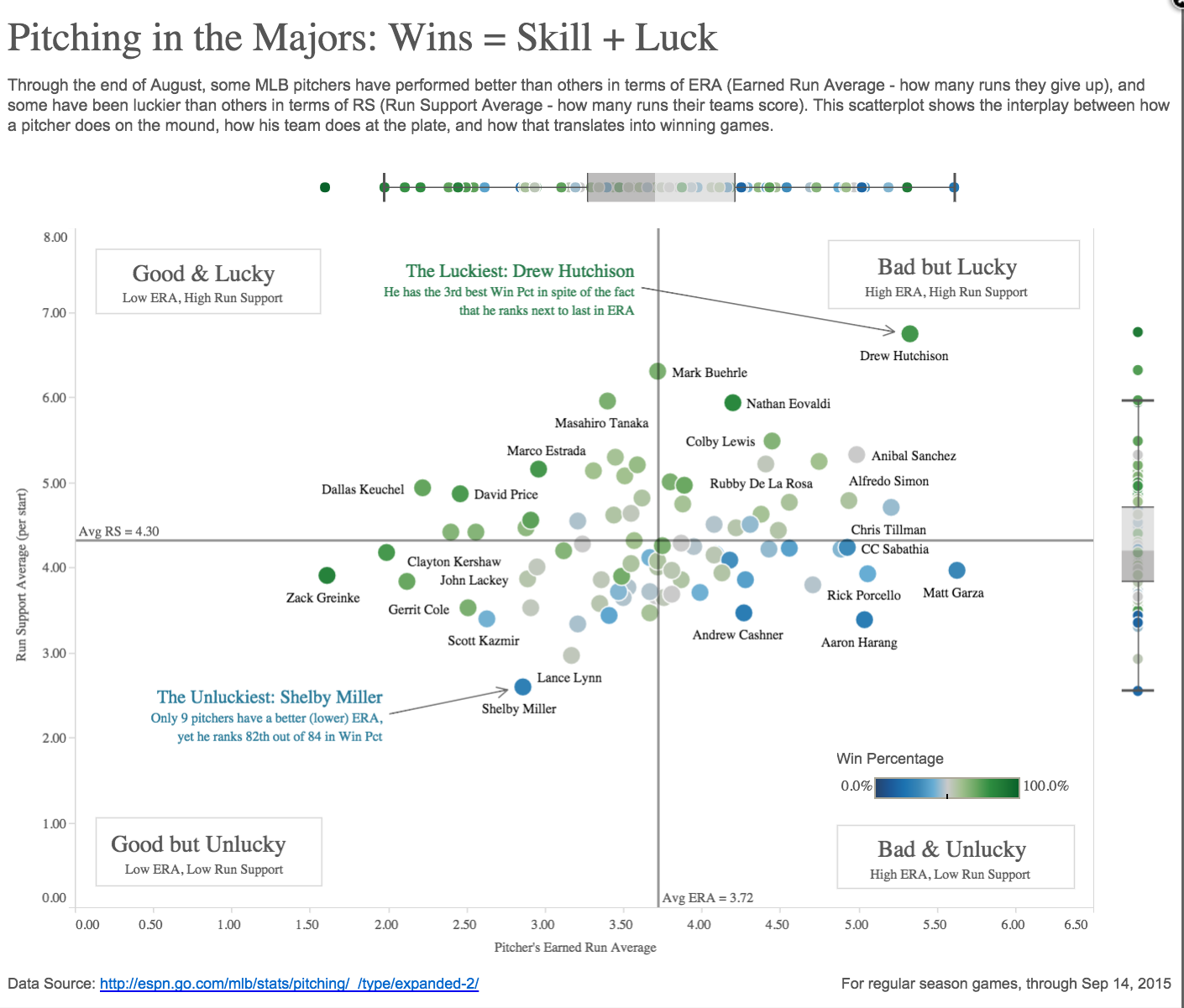
Scatter plots are my favorite visualization type, hands down. From my very first interactive data graphic about The Great One to the most recent visualization below on major league pitchers, I’ve learned a great deal from these Cartesian classics over the years. In this post I’ll show you how to make them even better than the standard ones in Tableau.
Iron Viz champ Shine Pulikathara published a scatterplot of NFL player heights and weights that included two marginal histograms, one for each axis. I tweeted that I liked it, and Lynn Cherny replied that it’s pretty common to see this kind of thing in R.
She’s right, and it turns out it’s also a common convention with other statistical graphing platforms like Matlab and Plotly. It’s called a scatterplot with marginal histograms. While Tableau has scatterplots and histograms as standard chart types, it doesn’t automatically combine them for you into a single view.
The goods news, though, is that it’s fairly easy to combine them using a dashboard with three sheets. There’s only one small trick to make the charts interact the way you want, which I’ll cover below. If you want to follow along, download 2015pitchingstats.xlsx.
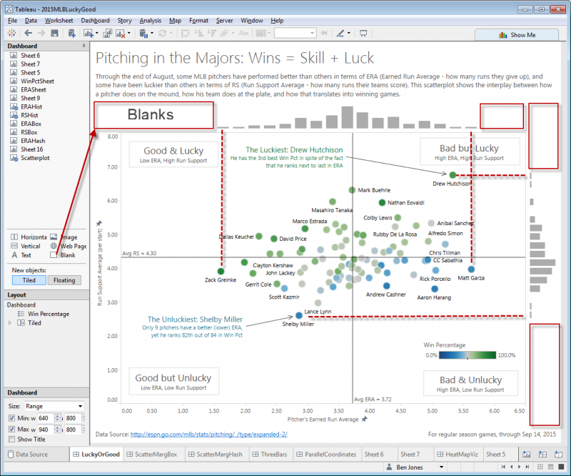
First, here is the finished version, showing pitchers' “skill” (Earned Run Average, or ERA) and “luck” (Runs Scored by their team, or RS) midway through the 2015 season:
Now, let’s consider the four easy steps to creating a scatterplot with marginal histograms:
Step 1: Create the Three Sheets
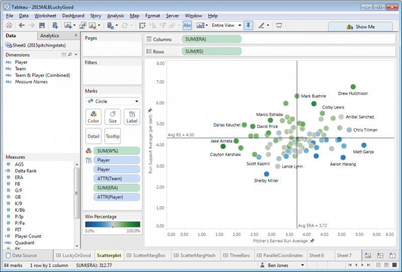
This part is fairly straightforward. Create a scatterplot and two histograms as three separate sheets in the same workbook. To create the scatterplot, drag ERA to columns, RS to rows, W% to color, Player to label, and then add two average reference lines, like this:
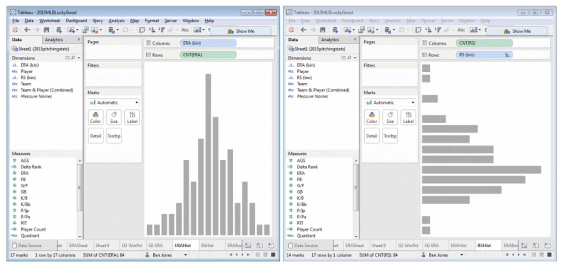
Next, to create the first histogram, create a new sheet, click on the Measure (say, ERA), click Show Me in the top right, and then choose Histogram. Do the same in another new sheet with RS, but click the Rotate icon in the top icon bar to flip the RS histogram 90 degrees. Notice that two new data fields appear in the Measures area: “ERA (bin)” and “RS (bin)." Right-click to edit these fields and change the “size of bins” to be 0.25 and hide the axes.
Step 2: Add the Histogram Bin Dimensions to the Scatterplot Chart Detail
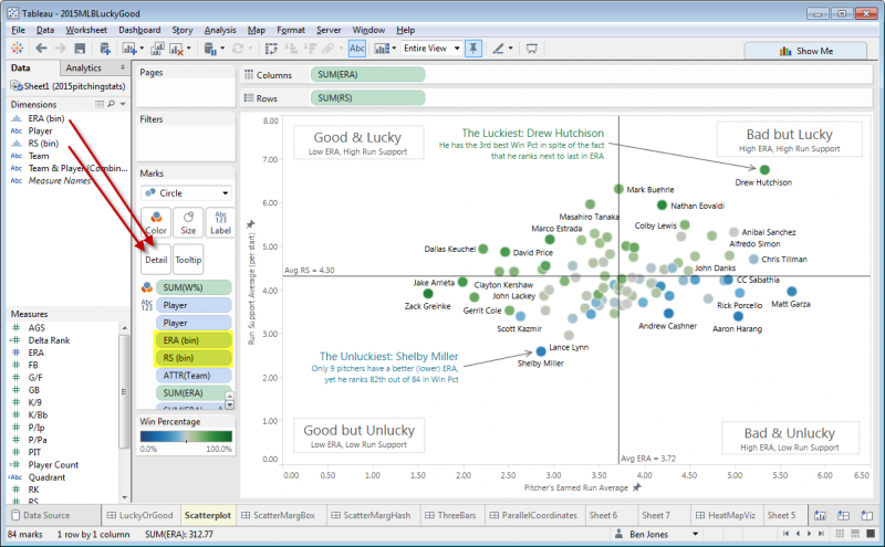
Without this step, you won’t be able to get the sheets to interact together in the dashboard. Go back to the scatterplot sheet you created in step 1 and drag both “ERA (bin)” and “RS (bin)” to Detail. You should now see these two fields listed in the Marks card area:
Step 3: Add the Three Sheets to a Dashboard
Next create a new dashboard and add the three sheets you created in step 1. Aligning the histograms with the scatterplot is the one messy part of this method. Add blanks to the left and right of the ERA histogram, and above and below the RS histogram. Drag the blanks until the extreme bars of the histogram align with the extreme points of the scatterplot:
Step 4: Create Two Highlight Actions
The last step is to get the sheets to interact with each other. There are lots of ways they could potentially interact, but here’s what I’d like to see happen:
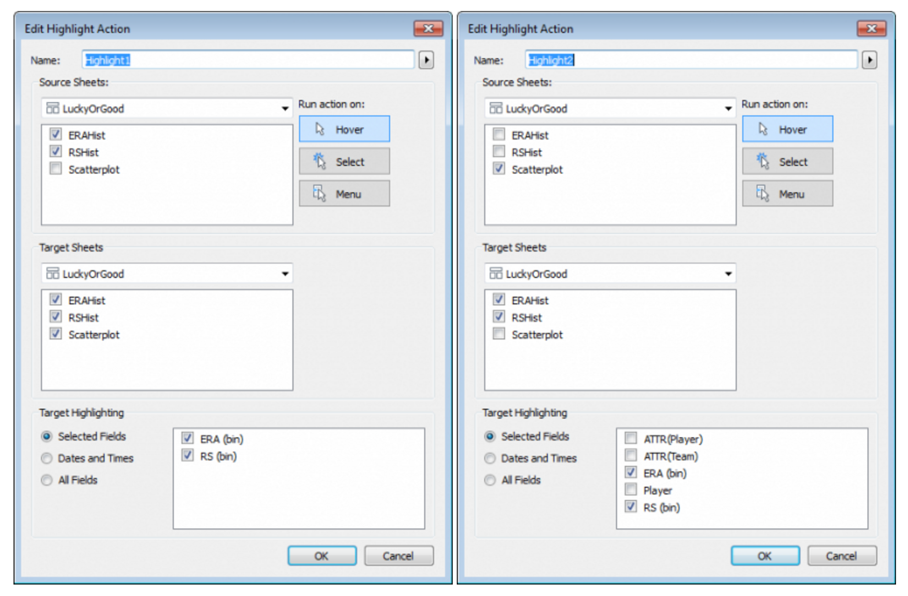
- When I hover my mouse cursor over any of the histogram bars, the corresponding circles on the scatterplot highlight.
- When I hover my mouse cursor over any of the scatterplot circles, the corresponding histogram bars highlight.
To do this, create two new dashboard actions by clicking Dashboard > Actions > Add Action > Highlight, and fill out the dialog boxes as follows:
That’s it! For finishing touches, I added a title, lead-in paragraph, data source and last accessed note, four area annotations to define the four quadrants, and two mark annotations to call out points of interest. I also edited the two average reference lines to uncheck “show recalculated line for highlighted or selected data points." This was strictly a matter of preference, and you may not decide to modify the reference lines in that way.
Other Variations
Here are a couple other variations that don’t involve the binning concept inherent in histograms and therefore don’t required step 2 above:
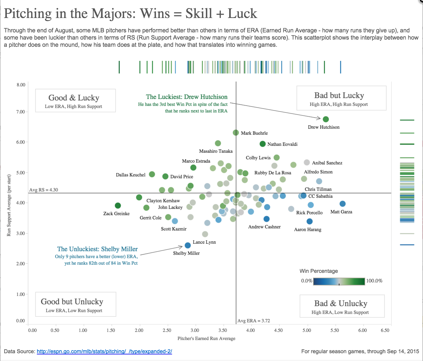
Scatterplot with Marginal Box-and-Whisker-Plots
Scatterplot with Marginal Hash Lines
Thanks for reading! I hope you found this helpful. Let me know if you have any further tips by leaving a comment. Also, I’m curious: Which of the three variations do you prefer?
For more tips, tricks, and works by Ben, check out his blog, DataRemixed, and his Tableau Public page.
Related Stories
Subscribe to our blog
Get the latest Tableau updates in your inbox.


